How Different Databases Store and Retrieve Data

A Simple Guide to Database Storage & Retrieval

Depending on whether you use a relational database like PostgreSQL, a document store like MongoDB, or a graph database like Neo4j, the same piece of data undergoes very different physical transformations before it is written to disk.

During retrieval, each database model also answers a different kind of question, shaped by how the data is stored, indexed, and accessed under the hood.

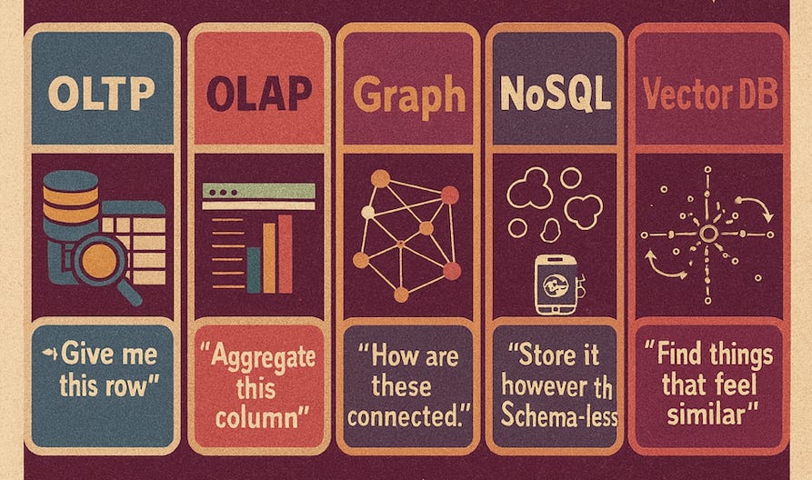
In this post, we focus on how data is physically stored by different database engines. Using a single example, a User Order, we will trace how it is stored and retrieved across five different database paradigms.

The Example Data: A User Order

To keep things consistent, let’s imagine we are storing this simple logical record:

• User: Alice (ID: 101)

• Order ID: 500

• Items: [“Keyboard”, “Mouse”]

• Total: $120

1. Relational Database

• The Architecture: Heap Files, Pages, and Tuples

• Examples: PostgreSQL, MySQL, SQL Server

• Purpose: Fast inserts & updates

In a relational ( OLTP ) database , data is stored in a Row-Oriented fashion and data lives in a structure known as a Heap File. This file is divided into fixed-size blocks called Pages (usually 8KB).

Physical Representation:

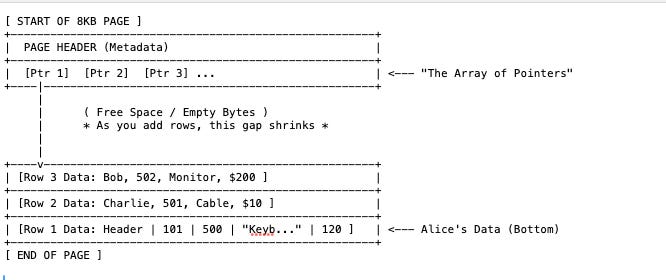
Row 1 → [Header Info] [101] [500] [”Keyboard, Mouse”] [120]

Header contains metadata like is this row locked? or is it deleted?

Retrieval:

The database uses an index (like a B-Tree) to find the correct Page Number. It loads that entire 8KB page into memory (RAM) and scans the offsets to read Alice’s order.

2. Columnar Database

• The Architecture: Column-Oriented Files & Vectorized Compression

• Examples: BigQuery, Snowflake, Redshift, ClickHouse

• Purpose: Analytics & aggregations

If Relational databases are “Row Stores,” these are “Column Stores.” They are the gold standard for analytics (OLAP) because they completely flip the physical layout.

Physical Representation:

• Vertical Partitioning: Instead of writing Alice’s entire order together, the database splits the order into separate physical files (or column chunks) for each attribute.

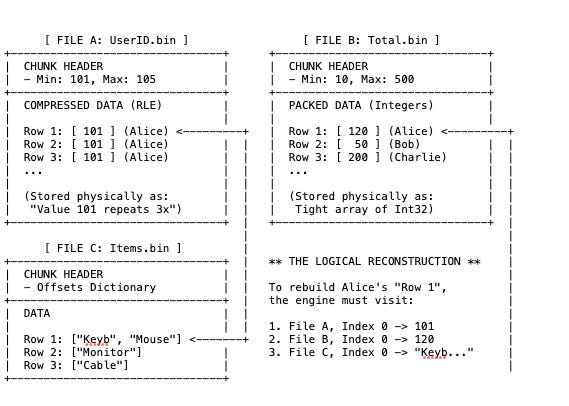
File A (User IDs): Stores [101, 102, 101, ...]
File B (Totals): Stores [120, 50, 120, ...]
File C (Items): Stores [”Keyboard”, “Mouse”, “Monitor”, ...]

• Aggressive Compression: Because File A contains only integers (User IDs), the database can use aggressive encoding. If Alice (101) made 50 orders in a row, it doesn’t write “101” 50 times. It uses Run-Length Encoding (RLE) to store something like 101 x 50. This shrinks the data footprint massively compared to row-based storage.

Image source: https://www.fastpix.io/blog/what-is-run-length-encoding

Retrieval:

SELECT SUM(Total) FROM Orders

If you run a above query, It will Ignores File A and File C entirely. It only loads File B. It reads the array of integers [120, 50, 200] and adds them up in a single CPU cycle.

3. Graph Database

• The Architecture: Fixed-Size Records & Linked Lists

• Examples: Neo4j, Neptune

• Purpose: Relationships-first queries

Graph databases split data into three specific files: one for Nodes, one for Relationships, and one for Properties. Physically, the data is stored as a Doubly Linked List.

Physical Representation:

Fundamentally, records in the Node and Relationship stores are fixed-size (for example, exactly 15 bytes or 34 bytes). This allows the database to calculate the exact disk offset of a record instead of searching for it.

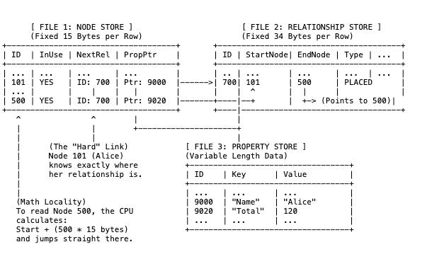
• The Node Store (File 1): This file is very small. It doesn’t contain the name “Alice” or the cost “$120”. It contains only Topology. i.e Row 101 (Alice): contains a pointer saying, “My first relationship is at ID 700.”

• The Relationship Store (File 2): This acts as the physical bridge.Row 700: says, “I connect Node 101 and Node 500.” It acts like a glue record.

• The Property Store (File 3): This is where the data lives. The Node Store points here just to retrieve the label “Alice”.

Retrieval:

If we want to find Alice’s Orders, they does not scan an index. They avoid “Indexes” for traversing relationships and instead use physical pointers, a concept known as Index-Free Adjacency.

Step 1: Get Node 101: The database knows that in the Node File, every record is exactly 15 bytes big. It multiplies 101 * 15 bytes to jump to the exact spot on disk for Alice ( byte #1515 )

The Analogy: The School Lockers

Imagine a long hallway with infinite lockers. Every single locker is exactly 15 inches wide. You want to open Locker #101.

Since you know every locker is exactly 15 inches, you don’t need to walk or look. You can calculate the exact distance from the front door.

Distance = Locker Number × Width
Distance = 101 × 15 inches = 1,515 inches.

You can put on a blindfold, walk exactly 1,515 inches, stop, and you will be standing exactly in front of Locker #101. You didn’t have to look at lockers 1 through 100.

Step 2: Read NextRel: Inside Alice’s record (at byte 1,515), there is a number : 700.
This number is a pointer. It implies: “relationship data is in #700 in the Relationship store.”

Step 3: Jump to Rel 700: Now switches to the Relationship File. In this file, every record is exactly 34 bytes big.

It multiplies 700 * 34 bytes to jump to the relationship record ( Byte #23,800 )

Step 4: Read EndNode: Inside that relationship record (at byte 23,800), it reads the data. It says: “connect to Node #500.”

Step 5: Jump to Node 500: It jumps directly to the Order node ( Node file ).

It multiplies 500 * 15 bytes to jump to the order data ( Byte #7,500 )

There is no “Searching” here. It is just jumping. Hence, It is O(1) complexity. This is why Graph databases are blazing fast for deep hierarchies but expensive to update (because you have to update multiple linked pointers).

4. Vector Database

• The Architecture: HNSW Graphs (Hierarchical Navigable Small World)

• Examples: Pinecone, Weaviate, Chrome

• Purpose: Similarity search (AI, embeddings)

In a vector database, Alice’s order (“Keyboard & Mouse”) is first converted by an AI model into an embedding, a high-dimensional vector represented as a long list of floating-point numbers (for example, [0.12, -0.98, 0.05, …]).

---

If embeddings interest you, I’ve explored them in more detail in a previous article.

Understanding Embeddings in LLMs

---

Physical Representation:

The database stores this in two parts:

1. The Vector Store: The raw lists of numbers (often compressed/quantized).

2. The HNSW Index: A multi-layered graph that acts like a “zoom-in” map.

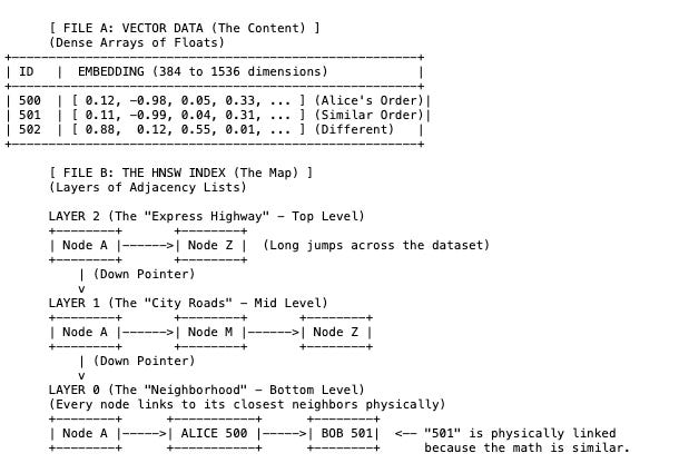
The Embedding: Alice’s order is no longer text. It is a mathematical coordinate.

The Layers (HNSW):

• Layer 2 (Top): Contains very few points. It allows the search algorithm to jump across the massive dataset quickly.

• Layer 0 (Bottom): Contains all the data points. Here, Alice’s vector is physically linked to Bob’s vector (501) not because they have sequential IDs (500, 501), but because their content is similar (both bought electronics).

Retrieval:

You don’t search for an exact ID like “500”. Instead, you provide a query vector (for example, “computer accessories”) which is the whole point of using a vector database.

The Analogy: Zooming In

Think of the HNSW Index like Google Map. 
You want to find a specific Coffee Shop (the data), but you are starting from space.

Layer 2 (The Satellite View): You can only see continents. You jump to United Kingdom (the closest “signpost” to your destination).

Layer 1 (The City View): You zoom in. Now you can see cities. You jump to London.

Layer 0 (The Street View): You zoom all the way down. Now you are on the ground. You check the buildings on the block and find the Coffee Shop.

1. Entry: The database has 3 “Signposts”: Clothes, Books, Technology.

   It looks at your search (“computer accessories”) and sees it is closest to Technology. It jumps there.

2. Descend: Inside “Technology,” it has 3 smaller signposts: Software, Hardware, Accessories. It sees your search is closest to Accessories. It jumps there.

3. Local Search: Now it looks at the actual items: Mouse, Charger, Monitor.

   It finds Alice’s order ( “Mouse”) because it is mathematically “close” to your query.

5. Document Database

• The Architecture: B-Tree Leaf Pages & BSON (Binary JSON)

• Examples: MongoDB, Couchbase, Amazon DocumentDB

• Purpose: Flexible schemas and hierarchical data

In a relational database, the column name “Total” is stored once in the table definition. In a Document database, “Total” is physically written inside every single record on the disk.

Physical Representation:

The data is stored in B-Tree Leaf Pages. Inside these pages, your JSON document is converted into BSON (Binary JSON), a format that includes length prefixes and type markers.

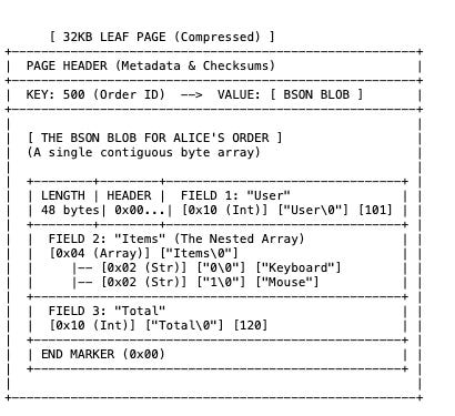
1. The Container (Leaf Page): MongoDB groups documents into large pages (often 32KB). These pages are usually compressed (using Snappy or Zlib) before being written to disk. To read Alice’s order, the CPU must load this 32KB block and decompress it in RAM.

2. Self-Describing Data: Look at “Field 3”. Every document can have different fields. Alice can have a “Total,” but Bob can have a “Discount” field instead. This takes up more space because repeat the word “Total” many times.

3. Data Locality (The Array): Look at “Field 2”. The items “Keyboard” and “Mouse” are physically glued to the Order ID. you get the whole order structure in one disk read.

Retrieval:

1. B-Tree Traversal: It navigates a B-Tree index to find the Leaf Page containing Key 500.

2. Decompression: It loads the Page and unzips it.

3. Scan: It reads the Length integer at the start of the BSON blob. It knows exactly how many bytes to grab to get the full object.

Your data is a Self-Contained Package. It carries its own field names and structure. This makes “Reads” incredibly fast (one seek gets everything, including nested lists), but makes “Storage” heavier (due to repeating field names).

---